Introduction
Meta-analysis in its present form of statistically integrating information from several studies all with a common underlying theme has been around for over 30 years. The medical, industrial and basic science fields have seen many attempts by many researchers to pull summary data together from various sources within a discipline with the goal of making some definitive statement about the state of the science in that discipline. Likewise authors of manuscripts in the background and rationale section of their paper always summarize what they believe to be the state of affairs up to the time of the presentation of their own results in that particular paper. The new data and results they present in their current publication is an attempt to update the progress in that field. Thus in a sense they have performed a partial meta-analysis of summarizing information from the past, presenting their added contribution and thus updating the knowledge base. They have not quite integrated past data in a rigorous statistical way with their new data, but have merely used the data history to justify their current research which pretty much stands on its own.
Thus meta-analysis is an after the fact attempt to pull together the current knowledge base whether it be publications or raw data and present a statistical synthesis of all the information and reach a conclusion as to the best treatment or intervention strategy based on all these past contributions. As stated by Glass (1) “Meta-analysis refers to the analysis of analyses...the statistical analysis of a large collection of analysis results from individual studies for the purpose of integrating the findings”.In most disciplines the statistical analysis can be endpoints such as mean effects, response rates, odds ratios, correlations, etc. We want to present the statistical issues of meta-analysis by example. We cannot possibly cover all the endpoints in this manuscript. We will thus concentrate on the continuous endpoint of mean effects with the understanding that the statistical concepts are transparent to other continuous endpoints such as correlations and to categorical endpoints such as odds ratios, relative risks and response rates. We begin by discussing the sources of literature review for a meta-analysis. The remainder of the manuscript will address the statistical terminology and approaches to conducting a meta-analysis. We then present techniques for investigating publication bias and conclude with some thoughts on the advantages and limitations of meta-analyses. Our discussions involve the major objectives of meta-analysis and are certainly detailed but not exhaustive as the meta-analytic field is quite extensive involving alternative statistical techniques not discussed here such as Bayesian and non parametric procedures as the available literature attests.
Systematic Reviews
One naturally starts out with a question such as “Do statins reduce the risk of cancer?” or “Is plasma vitamin C an appropriate biomarker for vitamin C intake?” There has to be a resource to search the literature to determine if one can synthesize the published or reported results and reach a definitive conclusion. This is called the “systematic review” or a review that clearly describes the methods used to locate, appraise and, where appropriate, combine relevant studies. The systematic review can have several key elements which include: 1) preparation for systematic reviewing or formulating the research question, 2) systematic research of the primary literature, 3) selection of papers for review and, 4) critical appraisal of the selected literature. The most common literature search sources are MEDLINE (United States Library of Medicine database), EMBASE (medical and pharmacologic database by Elsevier publishing), CINAHL (cumulative index to nursing and allied health literature), CANCERLIT (cancer literature research database)and the Cochrane Collaborative (an international nonprofit and independent organization which provides up-to-date, accurate information about the results/effects of healthcare worldwide. It produces and disseminates systematic reviews of healthcare interventions and in addition supports the search for evidence based information in the form of clinical trials and other studies of interventions.)
Thus all, these sources have played an important part in bringing information together so that researchers can be exposed to the availability of results from research directed at a common endpoint. The statistical synthesis, either quantitatively or qualitatively, of the results of the studies included in the systematic review and interpretation of the data is the actual meta-analysis. In most areas of research the statistical endpoints can be mean effects, response rates, odds ratios, correlations, etc. Thus, hopefully, one is aware of the selection of studies, the methods of data collection and how the results were statistically summarized and the conclusions derived. The methods for including studies in a meta-analysis can be extensive and suffice it to say, since our purpose is to address the statistical issues we will assume that the studies are addressing a common question, have well established eligibility criteria and the evaluation techniques for the endpoints are systematically established across the studies. One inclusion criteria in the meta-analysis in the clinical setting to be aware of is that the studies making comparisons of a treatment of interest to a control are properly randomized.
Effect sizes
An effect size in a single study is the measure of the difference of two treatment effects. For example in a single study where one wants to compare the mean reduction in blood pressure of a new anti hypertensive treatment, A, and the control treatment, B. The sample effect size (ES) is
ES= c(m)[(MA – MB)/S],
where MA is the mean reduction in blood pressure on treatment, A, and MB is the mean reduction in blood pressure on treatment, B and S is the pooled standard deviation from the both samples. The pooled standard deviation is defined as
S= { [ (nA -1)(sA)2 + (nB -1)(sB)2 ]/ (nA + nB -2)}1/2,
where sA and sB are the standard deviations (2) from samples A and B, respectively, and nA and nB are the sample sizes for A and B, respectively. The value c(m) is a correction factor (3) for the bias in estimating the true ES due to small sample sizes. It is defined as
c(m)= 1-3/(4m-1),
where m= nA + nB -2. One can see that as the sample size increases c(m) converges to the value 1. The variance of the study ES is sometimes estimated as (3)
var (ES)= [(nA + nB)/ nA nB] + (ES)2 /(2T-3.94),
where T= nA + nB. The approximate constant 3.94 is a correction factor (3) in this type of calculation.
Now let us assume we have many studies, k > 6, comparing some form of treatment A with a control. Please note that in meta-analyses we are not assuming that the treatment A is in the same form across all studies. For example in one study it may be A with exercise and in another A with a vitamin supplement, in another just A alone etc. The control in each may not be the same as long it is not A. That is to say, the control in one study may be a placebo tablet, in another it may be exercise alone, in another no intervention at all (if ethically this can be done), etc. The point being, in a meta–analysis you are asking the question whether receiving A in any form shows superiority in reducing blood pressure when it is compared to something other than A. Thus assuming we have k studies that we want to synthesize, a meta-analysis combines the k effect sizes, ES1, ES2,……..,ESk resulting in a mean effect size, ESmean,
ESmean = ∑i=1,k wi ESi /∑i=1,k wi for i=1,…,k.
Note the values, wi for i = 1,…,k. These are weights. In a meta-analysis, not all studies should be weighted equally. For example, a study containing 500 subjects should be weighted more than a study containing 80 subjects due to the added information. Weights can be determined in other ways such as the amount of follow up in longitudinal studies. A study in which the endpoint is time dependent such as survival and where subjects are followed for 10 years should de weighted more than a study in which subjects are only followed for 5 years. The actual calculations for determining weights can be quite complicated. One common technique is to allow the weight to be the inverse variance of the effect size (3) which we defined above i.e,
wi = 1/variance(ESi), i=1,…,k.
One rationale being that larger studies will have more precision and thus smaller variation and therefore greater weight. Another alternative choice for the simple weight would be the proportion of subjects in that study that contribute to the meta-analysis. For example, if N is the total number of subjects from all the studies contributing to the meta-analysis and Ni is the total number in study i, i = 1,…..,k, then N = N1 + N2 +….+Nk. We then define wi = Ni /N for i = 1,…,k, as the weight of the ith study. One of the assumptions often made in a meta-analysis is that the between studies variation do not differ. Thus the weights defined above do not account for the between studies variation (4). This is called a fixed effects meta-analysis. To allow for the randomness between the studies or a random effects model we let
wi = 1/ [variance(ESi + τ2)], i=1,…,k,
where τ2 is the among study variation. The computation is complex and need not be shown to make our point. One can see that all our calculations can be quite involved computationally and most calculations are routinely done using statistical software. However, we now have all the elements to test the overall effect of the new treatment,A, versus the control, B, for the combined k studies. Suppose that d is the population value of the combined ESmean. The null hypothesis is that there is no difference between A and B in the combined analysis or H0: d = 0 versus the alternative hypothesis, HA: d ¹ 0. A 95% confidence interval (5) on the population mean is:
[ESmean -1.96τ, ESmean +1.96τ].
If this interval covers 0 then there is no significant effect due to A.
To demonstrate the concepts described above, let us consider the following example. Suppose we have nine studies with effect sizes comparing treatments A and B; 0.574, -0.642, 0.363, -0.840, -0.783, 0.833, 0.842, 0.803, -0.345. As one can see, 5 are positive, favoring A and 4 are negative favoring B. The ESmean = 0.086, t =0.109 for the fixed effects model and t= 0.243 for the random effects model. The fixed effects 95% confidence interval (CI) = (-0.127-0.299) and the random effects 95% CI = (-0.387-0.563). In both cases the interval covers 0 and there is no benefit to A from the 9 studies. One can also see that the random effects CI is wider than the fixed effects CI as it takes into account the added variation between the studies which we attribute to heterogeneity or some inherent differences among the studies. Clearly this is so as about half of the studies showed some superiority due to treatment A and the others showed an advantage due to treatment B.
Figure 1 is a Forest plot which graphs the effects sizes and their individual 95% confidence intervals. The resulting overall effect size is demonstrated by the means diamond at the base of the plot.
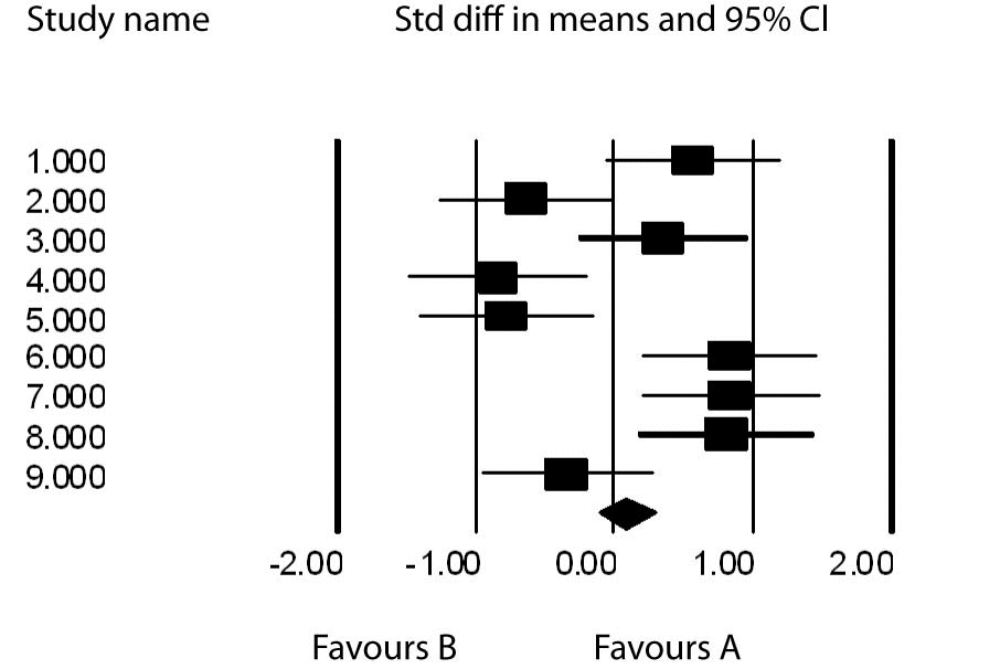
Figure 1. Forest plot of ES with their 95% confidence intervals.
Discussion of heterogeneity
The next task is to determine if there is significant heterogeneity among the studies. The statistic that we invoke is called the Q statistic and is used to determine the degree of heterogeneity. We do not compute it here. Suffice it to say, if Q is close to 0 then there is no heterogeneity. The Q has a chi square distribution (6) on k-1 degrees of freedom (df) or the number of studies minus one. Like other statistics we calculate Q and compare it to a critical value for the Chi square distribution. The null hypothesis is that there is no heterogeneity in the combined analysis or H0: Q=0 versus the alternative hypothesis, HA: Q¹ 0 implying there is significant heterogeneity. The critical value of the 9 studies for a chi square distribution on 9-1=8 df at an alpha level of 0.05 is 16.919. The calculated value of Q from our data is 38.897. Clearly the calculated Q is much greater than the critical value – over twice as much. Therefore we reject the null hypothesis and determine there is significant heterogeneity among our studies. This does not change our conclusion that there is no significant effect due to A. However, it does alert us that we should try to determine the source of the heterogeneity. Some possible sources of heterogeneity may be the clinical differences among the studies such as patient selection, baseline disease severity, management of inter current outcomes (toxicity), patient characteristics or others. One may also investigate the methodological differences between the studies such as mechanism of randomization, extent of withdrawals and lost to follow up or heterogeneity still can be due to chance alone and the source not easily detected. Quantifying heterogeneity can be one of the most troublesome aspects of meta-analysis. It is important because it can affect the decision about the statistical model to be selected (fixed or random effects). If significant heterogeneity is found then potential moderator variables can be found to explain this variability. It may require concentrating the meta–analysis on a subset of studies that are homogeneous within themselves. Let’s pursue this idea of heterogeneity one step further. Let’s examine the I2 index (6) which quantifies the extent of heterogeneity from a collection of effect sizes.
The I2 index can easily be interpreted as the percentage of heterogeneity in the system or basically the amount of the total variation accounted for by the between studies variance, τ2. In our example I2 = 79.433% or 79.4% of the variance or heterogeneity is due to τ2 or the between studies variance.
Publication bias
Funnel plots, plots of the studies’ effect estimates on the horizontal axis againstsample size in ascending order on the vertical axis, may be useful to assess the validity of meta-analyses. This is often referred to as “publication bias”. The funnel plot is based on the fact that precision in estimating the underlyingtreatment effect will increase as the sample size of the included studies increases. Results from small studies will scatter widelyat the bottom of the graph, with the spread narrowing among largerstudies to the top of the graph. In the absence of bias the plot will resemble a symmetricalinverted funnel. Conversely, if there is bias, funnel plotswill often be skewed and asymmetrical. Funnel plots are usually constructed as plotting the ES vs. the sample size or the ES vs. the SE.
In continuous data analysis we can use a linear regression approach (8) to measure funnel plot asymmetry on the ES. The ES is regressed against the estimate’s precision, the latter being defined as the inverse of the standard error (regression equation: ES=a+ b x precision, where a is the intercept and b is the slope). Since precision depends largely on sample size, small trials will be close to zero on the horizontal axis and vice versa for larger trials. The purpose is to not reject the null hypothesis that the line goes through the origin, i.e. intercept = 0. For our nine studies the funnel plot (not shown here) is symmetrical but rather flat as there are too few studies to result in a good plot. However, the symmetry is preserved as shown by the regression results. The test of the null hypothesis that the intercept equal to zero is not significant at the 0.05 alpha level indicates that the line goes through the origin. The actual p-value is 0.7747 indicating that there is strong evidence in the data to not support rejection of the null hypothesis of zero intercept. Thus there is no publication bias. Figure 2 is a funnel plot of 14 studies comparing two anti hypertensive therapies. The horizontal axis is the ES of the standard difference in means that we described above and the vertical axis is the standard error. One can see the symmetry. The studies with larger sample size or most precision are the dots or points located at the top of the graph and the studies with decreasing sample size or less precision (larger standard error) scatter towards the bottom of the plot. The diamond at the bottom of the plot is the means diamond for the overall meta-analysis comparing the two treatments and one sees it is close to zero. The statistical test for the intercept = 0 or the line goes through the origin is P = 0.730. The line is seen as the middle vertical line on the graph. The two angled lines give an outline of the pattern of points and one can see the funnel shape of the plot. Detailed discussions of funnel plots and test of symmetry can be found throughout the literature (8,9) pertaining to meta-analyses.
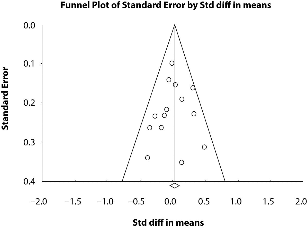
Figure 2. Funnel Plot of 14 studies with the effect size (Std diff in means) on the horizontal and the standard error on the vertical.
Conclusion
We have attempted here to give an overview of the major statistical approaches to meta-analysis. Advantages of meta-analyses are seen from the ability to address a controversial issue statistically that may not have been conclusively addressed in single studies. The ability to integrate results from diverse sources and address the relevant issues have been demonstrated many times in the literature through the publication of meta-analyses. One would want to certainly take advantage of the wealth of information published and have a rational way of synthesizing that information. There are certainly controversies (10) involved when one attempts to integrate information from various published works or different databases. Meta-analysis is prone to that controversy. However, every attempt is made to guard against bias through examination of topics such as heterogeneity and publication bias and to at least expose them and explain them. Limitations obviously result from selection of studies, choice of relevant outcome, methods of analysis, interpretation of heterogeneity and generalization and application of results. The statistical tools at hand are certainly adequate for addressing these issues. There are good online sources which provide guidelines for conducting a meta-analysis. These include CONDORT, QUORUM and MOOSE. These can be entered as key words to locate the resource. The Cochrane Collaborative mentioned above provides excellent guidelines as well. However, one should keep in mind that meta-analyses should not be a replacement for well designed large scale randomized studies (10) nor a justification for conducting small underpowered studies. It is a tool when properly utilized helps one to arrive at a reasonable and defensible decision from the scientific information already presented.