Introduction
One of the previous topics in Lessons in biostatistics presented the calculation, usage and interpretation of odds ratio statistic and greatly demonstrated the simplicity of odds ratio in clinical practice (1). The example used then was from a fictional study where the effects of two drug treatments to Staphylococcus Aureus (SA) endocarditis were compared. Original data are reproduced on Table 1.
Table 1. Results from fictional endocarditis treatment study by McHugh (1).
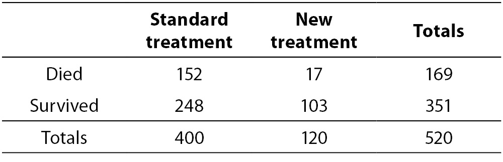
Following (1), the odds ratio (OR) of death of patients using standard treatment can be calculated as (152 x 103) / (248 x 47) = 3.71, meaning that patients at standard treatment present a chance to die 3.71 times greater than patients under new treatment. To a more detailed information about basic OR interpretations, please see McHugh (1). However, a more complex problem can arise when, instead of the association between one explanatory variable and one response variable (e.g., type of treatment and death), we are interested in the joint relationship between two or more explanatory variables and the response variable. Let us suppose we are now interested in the relationship between age and death in the same group of SA endocarditis patients. Table 2 presents the fictional new data. You ought to remember that those data are not real data and that the relationships described here are not meant to reflect any real associations.
Table 2. Results from fictional endocarditis treatment study by McHugh looking at age (1).
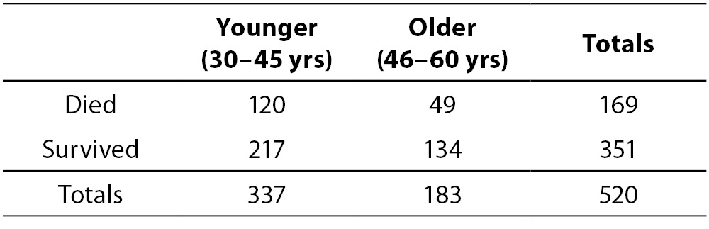
Again, we can calculate an OR as (120 x 134 / 217 x 49) = 1.51, meaning that the chance of an younger individual (between 30 and 45 years-old) death is about 1.5 times the chance of the death of an older individual (between 46 and 60 years-old). Now, instead, we have two variables related to the event of interest (death) at individuals with SA endocarditis. But in the presence of more than one explanatory variable, separately testing each independent variable against the response variable introduces bias into the research (2), Performing multiple tests on the same data inflates the alpha, thus increasing Type I error rates while missing possible confounding effects. So, how do we know whether the treatment effect on endocarditis result is being masked by the effect of age? Let us take a look at the treatment effect as stratified by age (Table 3).
Table 3. Effect of treatment on endocarditis stratified by age.
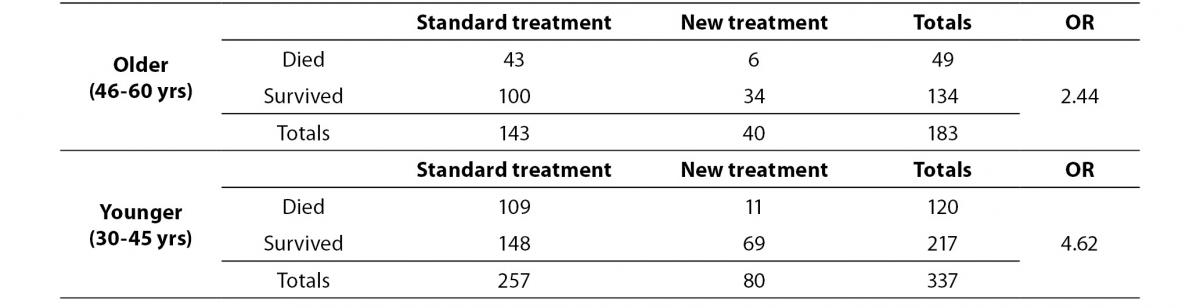
As table 3 illustrates, the impact of treatment is higher on younger individuals, because OR in the younger patients subgroup is higher than in the older patients subgroup. Therefore, it would be incorrect to simply look at the treatment results without considering the impact of age. The simplest way to solve this problem is to calculate some form of “weighted” OR (i.e., Mantel-Haenszel OR (3)), using Equation 1 below, where ni is the sample size of age class I, and a, b, c and d are the table cells, as presented by McHugh (1).
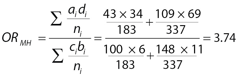 (1)
(1)It means that the weighted chance of death associated with standard treatment is 3.74 times the chance of death of individuals taking new treatment. However, as the number of explanatory variables increases, the complexity of these calculations can become nearly impossible to handle. Additionally, Mantel-Haenszel OR, like the simple OR, admits only categorical explanatory variables. For instance, to use a continuous variable like age we need to set a breaking point to categorize (in our case, arbitrarily set at 45 years-old) and could not use the real age. Determining breaking points is not always easy! But there is a better approach: using logistic regression instead.
Definition
Logistic regression works very similar to linear regression, but with a binomial response variable. The greatest advantage when compared to Mantel-Haenszel OR is the fact that you can use continuous explanatory variables and it is easier to handle more than two explanatory variables simultaneously. Although apparently trivial, this last characteristic is essential when we are interested in the impact of various explanatory variables on the response variable. If we look at multiple explanatory variables independently, we ignore the covariance among variables and are subjected to confounding effects, as was demonstrated in the example above when the effect of treatment on death probability was partially hidden by the effect of age.
A logistic regression will model the chance of an outcome based on individual characteristics. Because chance is a ratio, what will be actually modeled is the logarithm of the chance given by:
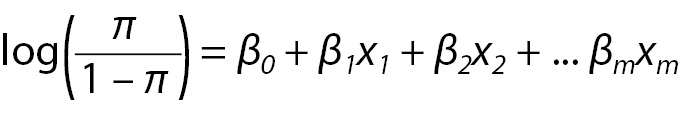 (2)
(2)where π indicates the probability of an event (e.g., death in the previous example), and βi are the regression coefficients associated with the reference group and the xi explanatory variables. At this point, an important concept must to be highlighted. The reference group, represented by β0, is constituted by those individuals presenting the reference level of each and every variable x1...m. To illustrate, considering our previous example, these are the individuals older aged that received standard treatment. Later, we will discuss how to set the reference level.
Logistic regression step-by-step
Let us apply a logistic regression to the example described before to see how it works and how to interpret the results. Let us build a logistic regression model to include all explanatory variables (age and treatment). This kind of model with all variables included is a called “full model” or a “saturated model” and is the best starting option if you have a good sample size and small number of variables to include (issues about sample size, variable inclusion and selection and others will be discussed in the next section. For now, we will keep it as simple as possible).
The result of our model can be seen below, at Table 4.
Table 4. Results from multivariate logistic regression model containing all explanatory variables (full model).

Now all we have to do is to interpret this output. Beginning with the intercept term, which corresponds to our β0. Taking the exponential of β0we have the mean odds to death of individuals in the reference category. So, exp(β0) = exp(-2.121) = 0.12 is the chance of death among those individuals that are older and received new treatment. A small difference in the interpretation of coefficients appears when we go to the next coefficients. Individuals that also received new treatment but are younger have a mean chance of death exp(β1) = exp(0.454) = 1.58 times the chance of reference individuals. Similarly, older individuals that received standard treatment have a mean chance exp(β2) = exp(1.333) = 3.79 times the chance of reference individuals to die. But what if individuals are younger and received standard treatment? Then we have to calculate exp(β1+β2) = exp(1.787) = 5.97 times the mean chance of reference individuals.
This is the basics of logistic regression interpretation. However, some issues appear during the analysis and solutions are not always readily available. In the next section we will discuss how to deal with them.
Logistic regression pitfalls
Odds and probabilities
First it is imperative to understand that odds and probabilities, although sometimes used as synonymous, are not the same. Probability is the ratio between the number of events favorable to some outcome and the total number of events. On the other hand, odds are the ratio between probabilities: the probability of an event favorable to an outcome and the probability of an event against the same outcome. Probability is constrained between zero and one and odds are constrained between zero and infinity. And odds ratio is the ratio between odds. The importance of this is that a large odds ratio (OR) can represent a small probability and vice-versa. Let us go back to our example to make this point clear.
The reference group (older individuals receiving new treatment) showed a chance of death approximately equal to 0.12. Using:  (3)
(3)
(3)it can be shown that the mean probability of death of this group is 0.11. Knowing that the mean chance of death in the group of younger individuals that received new treatment is 1.58 greater than the mean chance of the reference group, the chance of death to this group can be estimated as 1.58 x 0.12 = 0.19 or, using Equation 3 above, a probability of death equal to 0.16. Similarly, the mean chance of death of an older individual receiving standard treatment is 3.79 times the reference group, which means a chance of death equal to 3.79 x 0.12 = 0.45 or a probability of death equals to 0.31. Finally, younger individuals receiving standard treatment have a chance of death equal to 5.97 x 0.11 = 0.72 or a probability of death equal to 0.42.
Therefore, as demonstrated, a large OR only means that the chance of a particular group is much greater than that of the reference group. But if the chance of reference group is small, even a large OR can still indicate a small probability.
Continuous explanatory variables or variables with more than two levels
Now is time to think about what to do if explanatory variables are not binomial, as before. When an explanatory variable is multinomial, then we must build n-1 binary variables (called dummy variable) to it, where n indicates the number of levels of the variable. A dummy variable is just a variable that will assume value one if subject presents the specified category and zero otherwise. For instance, a variable named “satisfaction” that presents three levels (“Low”, “Medium” and “High”) needs to be represented by two dummy variables (x1 and x2) in the model. The individuals at reference level, let’s say “Low”, will present zeros in both dummy variables (Equation 4a), while individuals with “Medium” satisfaction will have a one in x1 and a zero in x2 (Equation 4b). The opposite will occur with individuals with “High” satisfaction (Equation 4c). Usually, statistical software does it automatically and the reader does not have to worry about it.
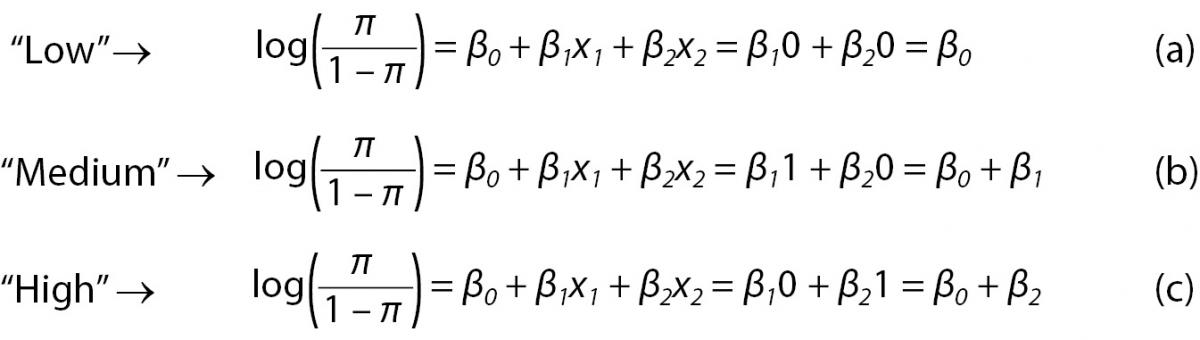 (4)
(4)While interpretation of outputs from multinomial explanatory variables is straightforward and follows the ones of binomial explanatory variables, the interpretation of continuous variables, on the other hand, is a bit more complex. The exp(β) of a continuous variable represents the increment of the chance of an event related to each unit increment on the explanatory variable. For instance, the variable “Age” in our previous example, if instead of being binomial (older x younger) were continuous, would produce the following result (Table 5).
Table 5. Results from multivariate logistic regression model containing all explanatory variables (full model), using AGE as a continuous variable.

The first thing to point out is that the “Age2” coefficient (Age here taken as a continuous variable) is now negative. It occurs because the older the individual (in years) the smaller the chance of death. If we take exp(-0.294) = 0.75, it shows us that for each year of life the chance to die of SA endocarditis decreases by 25%. The intercept, now, represents individuals that received the new treatment and with “zero years-old”. Take extra care when interpreting logistic regression results using continuous explanatory variables.
Variables inclusion and selection
A major problem when building a logistic model is to select which variables to include. Researchers usually collect as many variables as possible in their research instrument, then put all of them into the model and try to find something “significant”. This approach increases the emergence of two situations. First, one or more variables are statistically “significant”, but the researcher has no theory to link the “significant” variable to the event of interest modeled. Remember that you are working with samples and spurious results can occur. The second situation is that a model with more variables presents less statistical power. So, if there is an association between one explanatory variable and the occurrence of an event, researcher can miss this effect because saturated models (those that contains all possible explanatory variables) are not sensible enough to detect it. So the researcher must to be very cautious with the selection of variables to include into the model.
We can start a regression using either a full (saturated) model, or a null (empty) model, which starts only with the intercept term. In the first case, variables need to be dropped one by one, preferably dropping the less significant one. This is the preferred strategy just because is easier to handle, while the second requires all candidate variables to be tested each step in a way to select the better choice to include. On the other hand, if too many variables are included at once in a full model, significant variables could be dropped due to low statistical power, as mentioned above.
As a rule, if we have a large sample size, let’s say that we have at least ten individuals per variable, we can try to include all your explanatory variables in the full model. However, if we have a limited sample size in relation to the number of candidate variables, a pre-selection should be performed instead. One way to do that is to test all variables previously, using models with just one explanatory variable at a time (univariate models) and afterwards include in the multivariate model all variables that have shown a relaxed P-value (for instance, P ≤ 0.25). There is no reason to worry about a rigorous p-value criterion at this stage, because this is just a pre-selection strategy and no inference will derive from this step. This relaxed P-value criterion will allow reducing the initial number of variables in the model reducing the risk of missing important variables (4,5).
There is some debate about the appropriate strategy to variable selection (6) and the last is just another one. It is easy and intuitive. More elaborated methods are available, but whatever the method, it is very important that researchers get aware of the procedure applied and not just press some buttons on software.
Reference group setup
There are some explanatory variables for which the reference level is almost automatically determined. For instance, to our response variable named “Result” for which the outcomes are “died” and “survived”, the reference level is almost always set to “survived”, since the interest is focused on variables associated with the outcome, death.
On the other hand, some variables have no clear reference level, but present ordered levels and the reference level will be, usually, one of the endpoints or, less frequently, the central level. This is the case of variables assessed using Likert scales, a psychometric scale commonly involved in research that employs questionnaires (for instance, the degree of satisfaction about some product scaled as “satisfied”, “nor satisfied, nor unsatisfied” or “unsatisfied”). However, some variables have no ordered levels and no clear reference level. This can occur with geographic region. And then appears the question: what region should I use as reference?
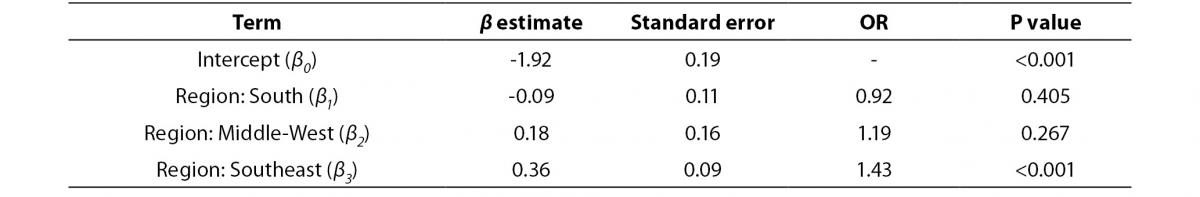
The answer is that there is no answer… However, reference level selection can change the model estimation in some cases. It is important to remember that all results (and significant effects) presented are relative to the reference level. To make this point clearer, let’s see an example. In a nationwide survey about the occurrence of diabetic ketoacidosis, individual’s geographic region was found to be significantly related to the probability of diabetic ketoacidosis at the onset of diabetes (7). In this work, north/northeast region was set as reference and southeast region was the only one to be statistically different relative to the reference. The results, showing just the region variable, are below (Table 6).
Table 6. Relationship between geographic region and ketoacidosis prevalence in Brazil (data from (7)). North/Notheast region used as reference level.
If we otherwise use Middle-East as the reference level, the next result will emerge (again, only geographic region is shown) (Table 7).
Table 7. Relationship between geographic region and ketoacidosis prevalence in Brazil (data from (7)). Middle-West region used as reference level.
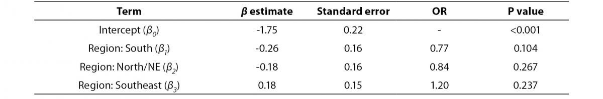
Finally, if we use the southeast region as reference level, we obtain following results (Table 8).
Table 8. Relationship between geographic region and ketoacidosis prevalence in Brazil (data from (7)). Southeast region used as reference level.

So, it is importance to pay attention to the setup of the reference levels. If there is no apparent rule derived by the data itself or by the prior knowledge about the variable values, one recommendation that remains is to select a reference level with minimum sample size, to allow adequate statistical power. Another recommendation that will make interpretation easier is to choose categories with the same relationship to the event of interest. If you believe that older individuals have smaller probability to die and people receiving new treatment are less probable to die, put these two categories as reference. You can use the opposite and set younger individuals and standard treatment. But choosing older individuals and standard treatment, although possible and not wrong, will difficult the interpretation of the results.
Conclusion
Logistic regression is a powerful tool, especially in epidemiologic studies, allowing multiple explanatory variables being analyzed simultaneously, meanwhile reducing the effect of confounding factors. However, researchers must pay attention to model building, avoiding just feeding software with raw data and going forward to results. Some difficult decisions on model building will depend entirely on the expertise of researcher on the field.
Acknowledgements
Author would like to thanks to Dr. Arianne Reis and Dr. Marcelo Ribeiro-Alves for the valuable manuscript revision and suggestions.