Introduction
Data analysis for research purposes usually aims to use the information gained from a sample of individuals in order to make inferences about the relevant population.
Statistical hypothesis testing is a widely used method of statistical inference. For example, if we are interested in whether there is a difference between men and women with respect to their serum cholesterol levels, or if the growth of bacteria follows some known distribution, or if our correlation coefficient is different from 0, we will use a hypothesis test. Computers and specialized statistical software, with their extensive help guides, make carrying out statistical tests rather easy. Statistical computer programs give the exact P value, and journal editors today demand that researchers quote actual P values, and let readers make their own interpretation (for example, see Instructions to Authors on Biochemia Medica web site).
On the other hand, there is more to interpretation of a test result than just stating “statistical significance” when P value is less then 0.05 or any other arbitrary cut-off value. So it is equally important for both, researchers and readers of scientific or expert journals, to understand statistical hypothesis testing procedures and how to use them when presenting or evaluating research results in the published article. There is one somewhat disregarded issue concerning statistical tests. Many published papers today quote rather a large number of P values which may be difficult to interpret (1). The purpose of this paper is to give a brief overview of basic steps in the general procedure for a statistical hypothesis testing, and to point out some common pitfalls and misconceptions.
Statistical hypothesis testing
A statistical hypothesis testing is a procedure that involves formulating a statistical hypothesis and using a sample data to decide on the validity of the formulated statistical hypothesis. Although details of the test might change from one test to another, we can use this four-step procedure to do any hypothesis testing:
1. Set up the null and alternative hypotheses.
2. Define the test procedure, including selection of significance level and power.
3. Calculate test statistics and associated P value.
4. Conclude that data are consistent or inconsistent with the null hypothesis, i.e. make a decision about null hypothesis.
Two possible errors can be made when deciding upon the null hypothesis (2).
Type I error occurs when we “see” the effect when actually there is none. The probability of making a Type I error is usually called alpha (α), and that value is determined in advance for any hypothesis test. Alpha is what we call “significance level” and its value is most commonly set at 0.05 or 0.01. When the P value, obtained in the third step of the general hypothesis test procedure is below the value of α, the result is called “statistically significant at the α level”.
Type II error occurs when we fail to see the difference when it is actually present. The probability of making the Type II error is called beta (β) and its value depends greatly upon the size of the effect we are interested in, sample size and the chosen significance level. Beta is associated with the power of the test to detect an effect of a specified size. More about power analysis in research can be found in one of the previous articles in Lessons in Biostatistics series (3).
What is the P value?
The P value is often misinterpreted as probability that the null hypothesis is true. The null hypothesis is not random and has no probability. It is either true or not. The actual meaning of the P value is the probability of having observed our data (or more extreme data) when the null hypothesis is true. For example, when we observe the difference in means of serum cholesterol levels measured in two samples, we want to know how likely it is to get such or more extreme difference when there is no actual difference between underlying populations. This is what P value tells us, and if we find that the P value is low, say 0.003, we consider the observed difference quite unlikely under the terms of the null hypothesis.
This leads us to the question of how low is low, i.e. the question of choosing the significance level.
Which significance level should we choose?
It is important to emphasize that significance level is an arbitrary value we choose as a cut-off value for deciding upon the null hypothesis and that it should be determined prior to analysis. Even when we do know the exact P value, we need some guidance about reaching a decision from the observed P value.
The plausible and simple solution is to identify the consequences of wrong decisions, i.e. of making the Type I or Type II error. If seeing (wrongly) a difference when actually there is none can be harmful for the population under study (or in general), we should choose a lower significance level, thus trying to minimize the probability of making the Type I error.
Picture the following scenario: A prospective clinical trial has shown that patients under treatment A experience considerable adverse effects. Treatment A was called off and the effects of a new treatment B were investigated. The decrease in adverse effects was observed for the new treatment B comparing to the old treatment A.
The question is: what significance level should we choose to estimate the significance of the observed difference, i.e. is the new treatment really better than the old one?
We can make two wrong conclusions, and each of them with consequence regarding patients.
Wrong conclusion #1: Treatment B is better, when actually it is the same as treatment A.
Consequence #1: We adopt the new treatment exposing patients to the adverse effects of Treatment B.
Wrong conclusion #2: Both treatments are the same, when actually treatment B is better than the treatment A.
Consequence #2: We do not adopt the new treatment in practice, but continue to search for a better solution.
Now it is quite obvious that making a Type I error (seeing the difference when there is none) in this scenario brings more harm to patients and that we should try to avoid making it.
When choosing the α significance level, we must bear in mind that if we decrease the value of α, the value of β will increase, thus decreasing the power of the test (3).
Can we “prove” the null hypothesis?
It may come as a surprise, but the answer to this question is very simple: No.
Getting an insignificant result about some treatment effect does not imply that there is none. The most we can say is that we failed to find sufficient evidence for its existence. To quote the title of an article in a highly respected medical journal - British Medical Journal: “Absence of evidence is not evidence of absence” (4). In terms of the null hypothesis we should say that “we have not rejected” or “have failed to reject” the null hypothesis (5). Statistical hypothesis test does not “prove” anything.
Multiple hypothesis testing
If we choose 0.05 as a significance level and then carry out 20 independent tests on the same data, the probability of making a Type I error when all underlying null hypotheses are in fact true is 0.64. This means that we are more likely to get one significant result than not. Furthermore, among 20 of such independent hypothesis tests, we expect to get 20 x 0.05 = 1 significant result purely by chance. How can this be?
The probability of making the Type I error (significance level) α can be described as probability of rejecting null hypothesis when the null hypothesis is actually true. We can also express it as:
α = 1 - (1 - α).
In this equation (1-α) is actually the probability of the complementary event, i.e. not rejecting the null hypothesis when the null hypothesis is actually true.
If we test several independent null hypotheses when all of them are actually true, the probability of making at least one Type I error equals 1- (probability of making none). In case of two tests that would be:
probability of making at least one Type I error =
α2= 1 - [(1-α) x (1-α)] = 1-(1-α)2.
α2= 1 - [(1-α) x (1-α)] = 1-(1-α)2.
When α=0.05, the probability of making at least one Type I error when testing two independent null hypotheses is:
α2 = 1 - 0.952 = 1 - 0.90 = 0.10.
For 3 tests, the probability of making at least one Type I error is:
α3 = 1 - 0.953 = 1 - 0.86 = 0.14.
In general, the probability of making at least one Type I error in the series of k independent null hypothesis tests when all null hypotheses are actually true is:
αk = 1-(1-α) k.
Now it is easy to see that for 20 tests the probability of making at least one Type I error when all null hypotheses are actually true equals 0.64. From Figure 1, we can see that it takes about 60 tests to reach the probability of 0.95 to get a significant result about some effect purely by chance, when no effect actually exists.
The expected number of significant results in a series of k independent hypothesis tests when all null hypotheses are actually true is simply calculated as:
k × α.
A problem of this kind arises when we perform hypothesis tests on multiple subsets of studied samples. In a study of association of back pain and risk of fatal ischemic heart disease (6) the author presented a table with age-specific mortality for men with and without back pain divided into two age groups and three groups by cause of death.
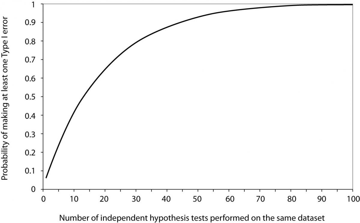
Figure 1. Probability of making at least one Type I error as a function of the number of independent hypothesis tests performed on the same dataset when all null hypotheses are true and significance level α is set to 0.05.
The results of the test comparing groups with and without back pain by means of P values were presented for each of the six subgroups plus two more for all causes in both age groups. Only one of those eight reported P values was less than 0.05 (0.02) while other ranged from 0.10 to 0.99. It was also pointed out that no association between back pain and any vascular disease was found in women, which leads to the notion that the author performed the same number of tests in the women subgroup. That would make the total of at least 16 tests among which only one was found to be “significant”, just about as many as we would expect to occur purely by chance.
The problem of multiple testing is common to microarray experiments (7). Let us consider the experiment of typing a series of random patients with a particular disease and a series of random controls without disease for a certain number of alleles. The number of tests would equal the number of alleles, testing whether each allele frequency was the same in the two populations. For 30 alleles, the probability of a false significant result when there is no association whatsoever is 0.76 while it increases to 0.92 for 50 alleles.
One way of dealing with these problems is to adjust either the minimum accepted significance level or to adjust P values obtained from the series of independent tests in order to preserve the overall significance level. If we adjust the minimum accepted significance level, we compare the “original” P values with the adjusted significance level. If we adjust P values, then we compare adjusted P values with the originally stated significance level.
A common way to adjust the original P values (sometimes called “nominal” P-values) for multiple testing is to use the Bonferroni method (1). By this method the adjustment is made by multiplying the nominal P values with the number of tests performed. So, if we made three independent tests which resulted in P values of 0.020, 0.030 and 0.040, the Bonferroni-adjusted P values would be 0.060, 0.090 and 0.120, respectively. While “original” results for all three tests would be considered significant at 0.05 level, after adjustment none of them remained significant.
Closely related to the Bonferroni method is the Šidak (Sidak) method (7). Šidak-adjusted P-values for k independent tests are calculated as:
pk = 1 – (1 – p) k.
Another problem occurs if we have multiple outcome measurements, in which case the tests will not be independent in general. Other multiple testing problems arise when we have more than two groups of study participants and wish to compare each pair of groups, or when we have a series of observations over time and wish to test each time point separately. For problems where the multiple tests are highly correlated, the aforementioned methods are not appropriate as they will be highly conservative and may miss the real effect (1).
The multiple testing problem is a serious problem in scientific research. Failure to adjust for multiplicity raises a serious doubt in obtained results because multiplicity inflates the significance level and diminishes the power of the research, and even more so if comparisons were not planned and prespecified. Thus, the multiplicity problem should not be taken lightly. Today there are numerous methods for adjusting multiplicity and an appropriate method should be implemented when facing the multiplicity problem. If we torture the data long enough they will finally produce something which is “significant”. But the significance will be unreliable, and conclusions based on those significant results are likely to be spurious.
Conclusion
Statistical hypothesis testing is a common method of statistical inference. There are several equally important issues not addressed in this article such as choosing the right test, performing one-tailed or two-tailed test, distinction of statistical significance and practical importance, just to name a few. It is important to a reader of scientific or expert journals as well as is to a researcher to understand the basic concepts of the testing procedure in order to make sound decisions about results and to draw accurate conclusions.
One more thing deserves attention when dealing with research results. Reporting a significant difference without reporting the size of the difference observed (i.e., the effect size) and associated confidence intervals is just half of the story. Thus, it is recommended to use both hypothesis testing and effect size estimation methods for statistical inference.